KFAC explained
Table of Contents
In this post
- I want to provide an intuitive explanation for the popular K-FAC (Kronecker-factorized curvature) approximation introduced in (Grosse & Martens, 2016; Martens & Grosse, 2015), using the concept of Hessian backpropagation (Dangel, Harmeling, et al., 2020).
- Based on this understanding, I want to explain how to generalize K-FAC for linear and convolution layers to transpose convolutions.
- Last but not least, I want to relate KFAC to other Kronecker approximations, specifically KFRA and KFLR (Botev et al., 2017).
This write-up accompanies the extension of Kronecker approximations to transpose convolution in BackPACK (Dangel, Kunstner, et al., 2020), which I have recently implemented.
Hessian backpropagation
All approximations we will talk about tackle the Hessian of a neural network's loss. Let \(f_{\vtheta}\) denote a neural network that maps a vector-valued input \(\vx\) to a vector-valued prediction \(\vf\), which is then scored by a convex loss function \(\ell(\vf, \vy) \in \sR\), using the ground truth (label) \(\vy\). The Hessian \(\nabla_{\vtheta}^{2} \ell\) collects the second-order derivatives of the loss w.r.t. the neural network's parameters \(\vtheta\) and has elements
\begin{align*} \left[ \nabla^{2}_{\vtheta}\ell \right]_{i,j} = \frac{\partial^{2} \ell}{\partial [\vtheta]_i \partial [\vtheta]_j}\,. \end{align*}More precisely, we will only be concerned with approximating certain blocks of this matrix. The block structure follows from the layer structure of our neural network. Assume that we have \(L\) layers with parameters \(\vtheta^{(1)}, \dots, \vtheta^{(L)}\) such that
\begin{align*} \vtheta = \begin{pmatrix} \vtheta^{(1)} \\ \vdots \\ \vtheta^{(L)} \end{pmatrix}\,. \end{align*}The Hessian inherits this structure and consists of \(L^2\) blocks, where block \((l_{1}, l_{2})\) contains all second-order partial derivatives w.r.t. parameters \(\vtheta^{(l_{1})}, \vtheta^{(l_{2})}\).
We only consider the blocks on the diagonal, which contain the second-order derivatives for parameters of the same layer, \(\nabla_{\vtheta^{(l)}}^2 \ell\). Such approximations of the Hessian are called block-diagonal approximations.
For feed-forward neural networks, these Hessian blocks can be obtained by backpropagating Hessian and gradient information through the network. Assume the network \(f_{\vtheta}\) consists of \(L\) layers \(f^{(l)}_{\vtheta^{(l)}}, l = 1, \dots, L\) such that
\begin{align*} f_{\vtheta} = f^{(L)}_{\vtheta^{(L)}} \circ f^{(L-1)}_{\vtheta^{(L-1)}} \circ \dots \circ f^{(1)}_{\vtheta^{(1)}}\,. \end{align*}The forward pass starts with \(\vz^{(0)} := \vx\) and produces the output \(\vz^{(L)} := \vf\) through hidden features \(\vz^{(l)}\) with the recursion (see Figure 1)
\begin{align*} \vz^{(l)} = f^{(l)}_{\vtheta^{(l)}}(\vz^{(l-1)}, \vtheta^{(l)}) \qquad l = 1, \dots, L\,. \end{align*}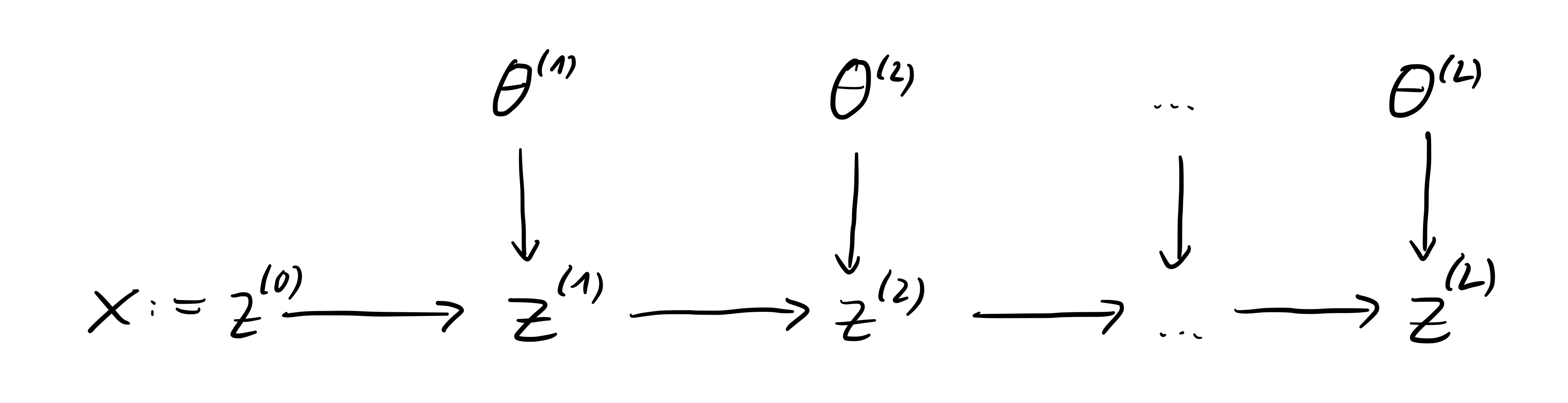
Figure 1: Forward pass of a feed-forward neural network.
The Hessian backpropagation equations to recover the per-layer Hessian are as follows (I will explain the symbols next):
\begin{align} \label{orglatexenvironment1} \nabla_{\vtheta^{(l)}}^{2}\ell &= \underbrace{ \left( \jac_{\vtheta^{(l)}}\vz^{(l)} \right)^{\top} \nabla_{\vz^{(l)}}^{2}\ell \left( \jac_{\vtheta^{(l)}}\vz^{(l)} \right)}_{\mathrm{(I)}} + \underbrace{ \sum_{k} \left(\nabla_{\vtheta^{(l)}}^{2} [\vz^{(l)}]_k \right) \left[\nabla_{\vz^{(l)}}\ell \right]_{k}}_{\mathrm{(II)}}\,. \end{align}This equation relates the Hessian w.r.t. the layer \(l\)'s output (\(\nabla_{\vz^{(l)}}^{2}\ell\)) to the Hessian w.r.t. to layer \(l\)'s parameters (\(\nabla_{\vtheta^{(l)}}^{2}\ell\)), which is the quantity we are seeking to approximate in this post:
- Let's first look at the second term (II). It contains second-order derivatives of the module's output w.r.t. its parameters. The parameterized layers we are interested in are linear layers, convolution layers, and transpose convolution layers. All these operations are linear in their parameters, hence the Hessian in (II), and therefore (II), vanishes for our discussion!
The first term (I) takes the Hessian w.r.t. layer \(l\)'s output, which is quadratic in \(\dim(\vz^{(l)})\), and applies the output-parameter Jacobian \(\jac_{\vtheta^{(l)}}\vz^{(l)} \in \sR^{\dim(\vz^{(l)}) \times \dim(\vtheta^{(l)})}\) from the left and right to obtain the parameter Hessian. This Jacobian stores the partial derivatives
\begin{align*} \left[ \jac_{\vtheta^{(l)}}\vz^{(l)} \right]_{i,j} = \frac{\partial [\vz^{(l)}]_{i}}{\partial [\vtheta^{(l)}]_{j}} \end{align*}and can easily be derived. We won't go into details of the Jacobian here; I'll simply provide you with its expression whenever necessary, see (Dangel, Harmeling, et al., 2020).
- For simplicity, we also won't discuss the details how to obtain the Hessian w.r.t. the layer output and simply assume that this can be done, see (Dangel, Harmeling, et al., 2020).
Equation \eqref{orglatexenvironment1} describes how to obtain the exact per-layer Hessian, and is the starting point for obtaining structural approximations to it.
KFAC
We will focus on the approximation of block-diagonal curvature through Kronecker products. To see how Kronecker structure emerges in the Hessian, we start with the linear layer.
Linear layer
Let's consider a linear layer (without bias for simplicity)
\begin{align*} \vz^{(l)} = \mW^{(l)} \vz^{(l-1)} \end{align*}with parameters \(\vtheta^{(l)} = \vec \mW^{(l)}\). The output-parameter Jacobian is
\begin{align*} \jac_{\vtheta^{(l)}}\vz^{(l)} = {\vz^{(l-1)}}^{\top} \otimes \mI_{\dim(\vz^{(l)})} \end{align*}and has Kronecker structure. This Kronecker structure carries through to the parameter Hessian: insertion into the Hessian backpropagation equation \eqref{orglatexenvironment1} yields
\begin{align*} \nabla_{\vtheta^{(l)}}^{2}\ell &= \left[ {\vz^{(l-1)}}^{\top} \otimes \mI_{\dim(\vz^{(l)})} \right]^{\top} \nabla_{\vz^{(l)}}^{2}\ell \left[ {\vz^{(l-1)}}^{\top} \otimes \mI_{\dim(\vz^{(l)})} \right] \\ &= \vz^{(l-1)} {\vz^{(l-1)}}^{\top} \otimes \nabla_{\vz^{(l)}}^{2}\ell\,. \end{align*}In KFAC, the second Kronecker factor is approximated through an outer product of a backpropagated vector \(\vg^{(l)}\) with \(\dim(\vg^{(l)}) = \dim(\vz^{(l)})\). The details of this vector don't matter here; just consider it "one way" to approximate \(\nabla_{\vz^{(l)}}^{2}\ell \approx \vg^{(l)} {\vg^{(l)}}^{\top}\).
We have arrived at the Kronecker-factored curvature approximation for linear layers:
\begin{align} \label{orglatexenvironment2} \mathrm{KFAC}(\nabla_{\vtheta^{(l)}}^{2}\ell) = \vz^{(l-1)} {\vz^{(l-1)}}^{\top} \otimes \vg^{(l)}{\vg^{(l)}}^{\top}\,. \end{align}Convolution layer
Next up, we consider a convolution layer (without bias for simplicity). It takes an image-shaped tensor \(\tZ^{(l-1)} \in\sR^{C_{\text{in}} \times H_{\text{in}} \times W_{\text{in}}}\) and maps it to an image-shaped output \(\tZ^{(l)} \in\sR^{C_{\text{out}} \times H_{\text{out}} \times W_{\text{out}}}\). The kernel is a rank-4 tensor \(\tW^{(l)} \in \sR^{C_{\text{out}} \times C_{\text{in}} \times K_{H} \times K_{W}}\), and we can write
\begin{align*} \tZ^{(l)} = \tZ^{(l-1)} \star \tW^{(l)} \end{align*}with \(\vtheta^{(l)} = \vec \tW^{(l)}\). Instead of tensors, we will view the forward pass in terms of the matrices \(\mW^{(l)} \in \sR^{C_{\text{out}} \times C_{\text{in}} K_{H} K_{W}}\) and \(\mZ^{(l)} \in\sR^{C_{\text{out}} \times H_{\text{out}} W_{\text{out}}}\), which are just reshapes of the above tensors. With these matrices, convolution can be expressed as matrix multiplication
\begin{align*} \mZ^{(l)} = \mW^{(l)} \llbracket\tZ^{(l-1)}\rrbracket \end{align*}
where \(\llbracket\tZ^{(l-1)}\rrbracket \in \sR^{C_{\text{in}} K_{H} K_{W} \times H_{\text{out}} W_{\text{out}}}\) is the unfolded input, sometimes also referred to as im2col. We don't have to worry how to obtain the unfolded input; deep learning libraries provide such functionality. Now, the forward pass looks already very similar to the linear layer.
To use the Hessian backpropagation equation \eqref{orglatexenvironment1}, we need to flatten the output into a vector, \(\vz^{(l)} = \vec \mZ^{(l)} \in \sR^{C_{\text{out}} H_{\text{out}} W_{\text{out}}}\). For this vector, the Jacobian is given by
\begin{align*} \jac_{\vtheta^{(l)}}\vz^{(l)} = \llbracket \tZ^{(l-1)} \rrbracket^{\top} \otimes \mI_{C_{\text{out}}}\,. \end{align*}Inserting this, we get
\begin{align*} \nabla_{\vtheta^{(l)}}^{2} \ell &= \left( \llbracket \tZ^{(l-1)} \rrbracket^{\top} \otimes \mI_{C_{\text{out}}} \right)^{\top} \nabla_{\vz^{(l)}}^{2} \ell \left( \llbracket \tZ^{(l-1)} \rrbracket^{\top} \otimes \mI_{C_{\text{out}}} \right) \\ &= \left( \llbracket \tZ^{(l-1)} \rrbracket \otimes \mI_{C_{\text{out}}} \right) \nabla_{\vz^{(l)}}^{2} \ell \left( \llbracket \tZ^{(l-1)} \rrbracket^{\top} \otimes \mI_{C_{\text{out}}} \right)\,. \end{align*}Unlike for the linear layer, this cannot be simplified to a Kronecker product without further approximations! (Grosse & Martens, 2016) present the assumptions under which the above expression simplifies to a Kronecker product.
I want to take a different approach here. It is relatively easy to see that if the \(C_{\text{out}} H_{\text{out}} W_{\text{out}} \times C_{\text{out}} H_{\text{out}} W_{\text{out}}\) matrix \(\nabla_{\vz^{(l)}}^{2} \ell\) could be expressed as a Kronecker product,
\begin{align*} \nabla_{\vz^{(l)}}^{2}\ell = \mA \otimes \mB\,, \qquad \mA \in \sR^{H_{\text{out}} W_{\text{out}} \times H_{\text{out}} W_{\text{out}}}, \mB \in \sR^{C_{\text{out}} \times C_{\text{out}}}\,, \end{align*}this would imply a Kronecker structure for the weight Hessian,
\begin{align*} \implies \nabla_{\vtheta^{(l)}}^{2}\ell = \llbracket \tZ^{(l-1)} \rrbracket \mA \llbracket \tZ^{(l-1)} \rrbracket^{\top} \otimes \mB\,. \end{align*}If we now fix \(\mA = \mI_{H_{\text{out}} W_{\text{out}}}\) (see Figure 2), and determine \(\mB\) by finding the best possible approximation to \(\nabla_{\vtheta^{(l)}}^{2}\ell\) (see Figure 3), we recover the Kronecker factors for convolutions as presented in (Grosse & Martens, 2016).
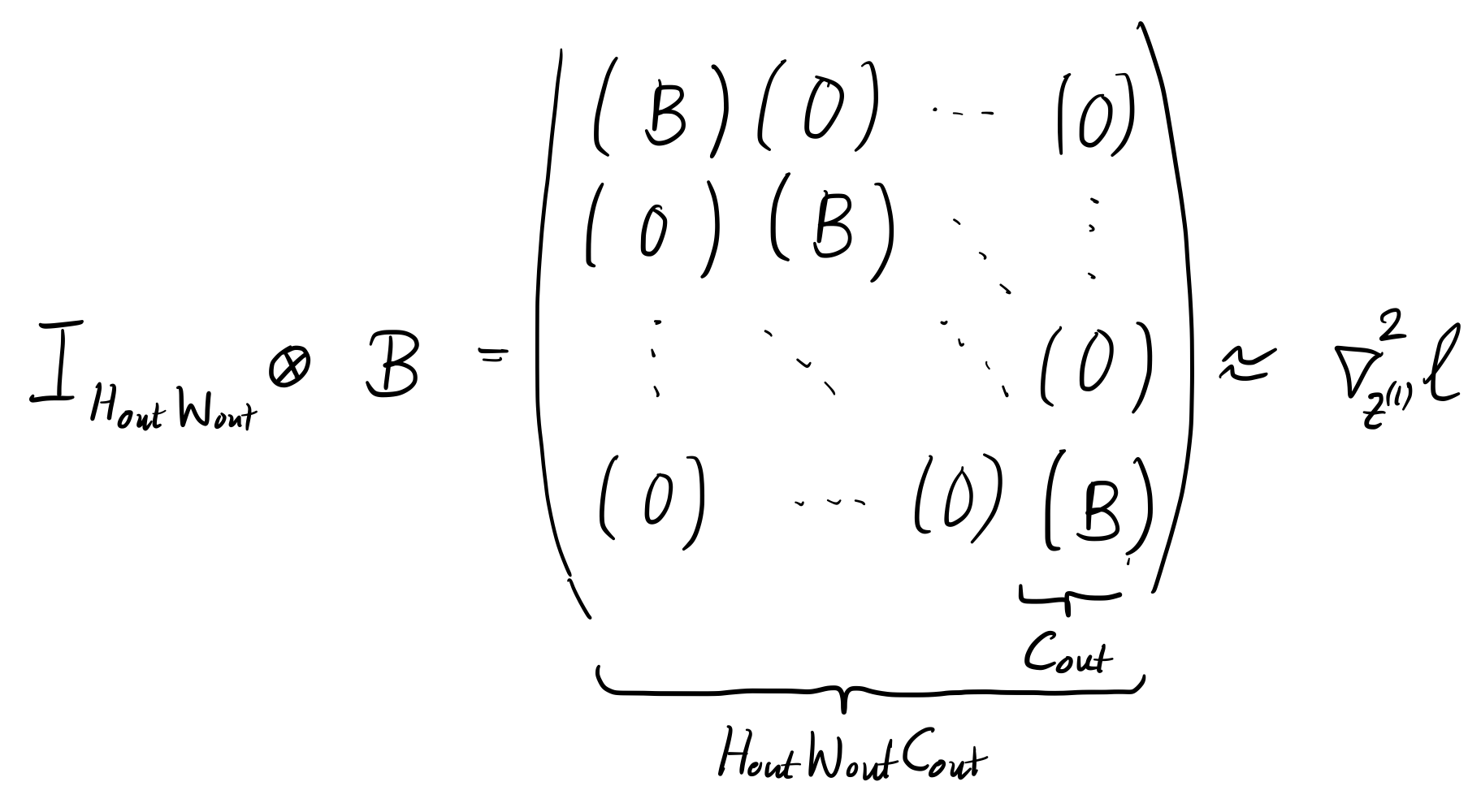
Figure 2: Imposed Kronecker approximation on the backpropagated Hessian to obtain a Kronecker-factored Hessian w.r.t. the weights of a convolution layer.
Concretely, we will minimize the squared Frobenius norm between \(\nabla_{\vz^{(l)}}^{2}\ell\) and \(\mI_{H_{\text{out} W_{\text{out}}}} \otimes \mB\) to determine the best choice for \(\mB\). From a high-level perspective, \(\mB\) is the mean over the \(C_{\text{out}} \times C_{\text{out}}\) diagonal blocks of \(\nabla_{\vz^{(l)}}^{2} \ell\), see Figure 3. To see this in more detail, let's write down the elements of \(\mI_{H_{\text{out} W_{\text{out}}}} \otimes \mB\). To address elements, we require 4 indices to distinguish channels from spatial dimensions. This yields
\begin{align*} \left[ \mI_{H_{\text{out}} W_{\text{out}}} \otimes \mB \right]_{(x_1, c_1),(x_2, c_2)} = \delta_{x_1,x_2} \left[ \mB \right]_{c_1,c_2}\,, \qquad x_{1,2} = 1, \dots, H_{\text{out}} W_{\text{out}}\,, \quad c_{1,2} = 1, \dots, C_{\text{out}}\,. \end{align*}The squared Frobenius norm of the residual between \(\nabla_{\vz^{(l)}}^{2}\ell\) and \(\mI_{H_{\text{out} W_{\text{out}}}} \otimes \mB\) is
\begin{align*} \left\lVert\nabla_{\vz^{(l)}}^{2}\ell - \mI_{H_{\text{out}} W_{\text{out}}} \otimes \mB \right\rvert_{F}^{2} = \sum_{x_1, x_2}\sum_{c_1, c_2} \left( \left[ \nabla_{\vz^{(l)}}^{2}\ell \right]_{(x_1, c_1), (x_2, c_2)} - \delta_{x_1,x_2} \left[ \mB \right]_{c_1, c_2} \right)^2 \end{align*}Taking the gradient w.r.t. an element of \(\mB\) we get
\begin{align*} \frac{\partial \left\lVert\nabla_{\vz^{(l)}}^{2}\ell - \mI_{H_{\text{out}} W_{\text{out}}} \otimes \mB \right\rVert_{F}^{2}}{ \partial \left[ \mB \right]_{\tilde{c}_1, \tilde{c}_2}} &= \sum_{x_1, x_2}\sum_{c_1, c_2} -2 \delta_{c_1,\tilde{c}_1} \delta_{c_2,\tilde{c}_2} \delta_{x_1,x_2} \left( \left[ \nabla_{\vz^{(l)}}^{2}\ell \right]_{(x_1, c_1), (x_2, c_2)} - \delta_{x_1,x_2} \left[ \mB \right]_{c_1, c_2} \right) \\ &= -2 \sum_{x} \left( \left[ \nabla_{\vz^{(l)}}^{2}\ell \right]_{(x, \tilde{c}_1), (x, \tilde{c}_2)} - \left[ \mB \right]_{\tilde{c}_1, \tilde{c}_2} \right) \\ &= 2 H_{\text{out}} W_{\text{out}} \left[ \mB \right]_{\tilde{c}_1, \tilde{c}_2} - 2 \sum_{x} \left[ \nabla_{\vz^{(l)}}^{2}\ell \right]_{(x, \tilde{c}_1), (x, \tilde{c}_2)}\,, \end{align*}and setting this gradient to zero, we arrive at the expression for an element of \(\mB\)
\begin{align*} \left[ \mB \right]_{c_1, c_2} = \frac{1}{H_{\text{out}} W_{\text{out}}} \sum_{x} \left[ \nabla_{\vz^{(l)}}^{2}\ell \right]_{(x, c_1), (x, c_2)}\,, \end{align*}i.e. we obtain \(\mB\) by average-tracing over the spatial dimension of the Hessian w.r.t. the output, see Figure 3 for an illustration.
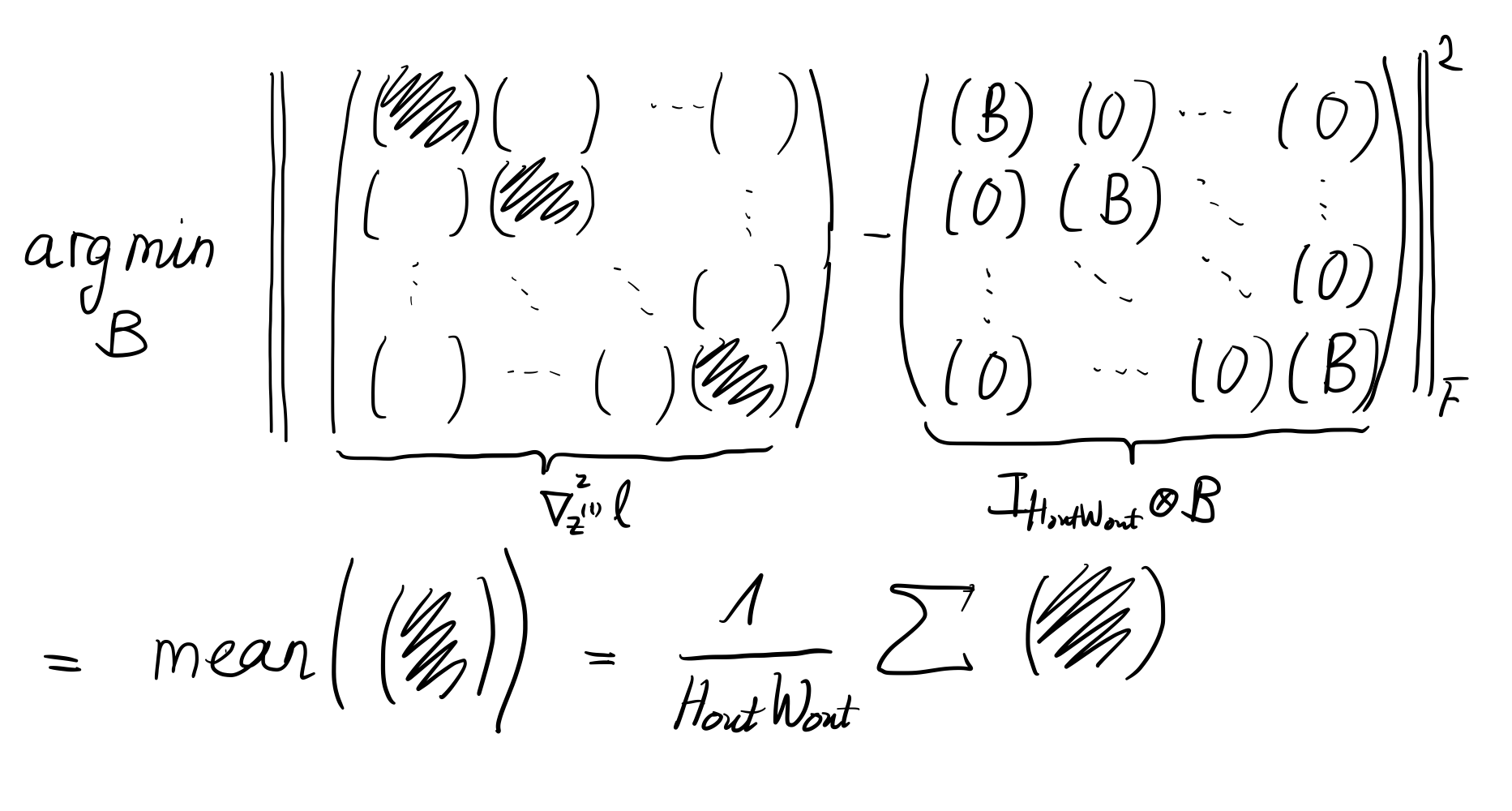
Figure 3: Illustration for finding the best approximation to the backpropagated Hessian with the imposed Kronecker structure.
As a last step, we will insert the approximation that KFAC uses for the backpropagated Hessian w.r.t. the convolution output. Just like for the linear layer, this is an outer product of vectors \(\vg^{(l)} \in \sR^{C_{\text{out}} H_{\text{out}} W_{\text{out}}}\) of same dimension as the output (again, it does not matter here how these vectors are obtained in detail). This leads to
\begin{align*} \left[ \mB \right]_{c_1, c_2} &= \frac{1}{H_{\text{out}} W_{\text{out}}} \sum_{x} \left[ \vg^{(l)} {\vg^{(l)}}^{\top} \right]_{(x, c_1), (x, c_2)} \\ &= \frac{1}{H_{\text{out}} W_{\text{out}}} \sum_{x} \left[ \vg^{(l)}\right]_{(x, c_1)} \left[\vg^{(l)} \right]_{(x, c_2)} \end{align*}which can be expressed as
\begin{align*} \mB = \frac{1}{H_{\text{out}} W_{\text{out}}} {\mG^{(l)}}^{\top} \mG^{(l)} \end{align*}were \(\mG^{(l)} \in \sR^{H_{\text{out}} W_{\text{out}} \times C_{\text{out}}}\) is a matrix-view of \(\vg^{(l)}\) that separates the spatial dimensions into rows, and the channel dimensions into columns.
We have now derived the Kronecker approximation for weights in convolution layers from (Grosse & Martens, 2016):
\begin{align} \label{orglatexenvironment3} \mathrm{KFAC}(\nabla_{\vtheta^{(l)}}^{2} \ell) = \llbracket \tZ^{(l-1)} \rrbracket \llbracket \tZ^{(l-1)} \rrbracket^{\top} \otimes \frac{1}{H_{\text{out}} W_{\text{out}}} {\mG^{(l)}}^{\top} \mG^{(l)}\,. \end{align}Note that, in contrast to the linear layer in Equation \eqref{orglatexenvironment2}, we had to make an additional approximation to the backpropagated Hessian to impose a Kronecker structure.
Transpose convolution layer
Transpose convolution is structurally quite similar to convolution. We will use this similarity to define a Kronecker-factorized Hessian approximation for its weight.
Just like a convolution layer, a transpose convolution layer maps an image-shaped tensor \(\tZ^{(l-1)} \in\sR^{C_{\text{in}} \times H_{\text{in}} \times W_{\text{in}}}\) to an image-shaped output \(\tZ^{(l)} \in\sR^{C_{\text{out}} \times H_{\text{out}} \times W_{\text{out}}}\) using a kernel, a rank-4 tensor, \(\tW^{(l)} \in \sR^{C_{\text{out}} \times C_{\text{in}} \times K_{H} \times K_{W}}\). We can write
\begin{align*} \tZ^{(l)} = \tZ^{(l-1)} \star_{\top} \tW^{(l)} \end{align*}with \(\vtheta^{(l)} = \vec \tW^{(l)}\), and using \(\star_{\top}\) to denote transpose convolution. Instead of tensors, we will view the forward pass in terms of the matrices \(\mW^{(l)} \in \sR^{C_{\text{out}} \times C_{\text{in}} K_{H} K_{W}}\) and \(\mZ^{(l)} \in\sR^{C_{\text{out}} \times H_{\text{out}} W_{\text{out}}}\), which are just reshapes of the above tensors. In complete analogy to convolution, transpose convolution can be expressed as matrix multiplication
\begin{align*} \mZ^{(l)} = \mW^{(l)} \llbracket\tZ^{(l-1)}\rrbracket_{\top} \end{align*}where \(\llbracket\tZ^{(l-1)}\rrbracket_{\top} \in \sR^{C_{\text{in}} K_{H} K_{W} \times H_{\text{out}} W_{\text{out}}}\) is the unfolded input for a transpose convolution. This unfolding operation \(\llbracket \cdot \rrbracket_{\top}\) only differs in low-level details from its counterpart \(\llbracket \cdot \rrbracket\) for convolution. We don't have to worry about how to obtain this unfolded input; there are libraries that provide such functionality.
Since the we have expressed the forward pass of transpose convolution in the same form as for convolution, we can fast-forward through all the intermediate steps and write down the approximation of KFAC for the kernel of a transpose convolution:
\begin{align} \label{orglatexenvironment4} \mathrm{KFAC}(\nabla_{\vtheta^{(l)}}^{2} \ell) = \llbracket \tZ^{(l-1)} \rrbracket_{\top} \llbracket \tZ^{(l-1)} \rrbracket^{\top}_{\top} \otimes \frac{1}{H_{\text{out}} W_{\text{out}}} {\mG^{(l)}}^{\top} \mG^{(l)}\,. \end{align}There is one caveat that you may have noticed already if you have ever worked with transpose convolutions in deep learning libraries like PyTorch: while the kernel for convolution is commonly stored as a \(C_{\text{out}} \times C_{\text{in}} \times K_{H} \times K_{W}\) tensor, the kernel for transpose convolution is usually stored in the permuted format \(C_{\text{in}} \times C_{\text{out}} \times K_{H} \times K_{W}\). To work with the Kronecker representation, we therefore need to properly pre- and post-process quantities to and from \(C_{\text{in}} \times C_{\text{out}} \times K_{H} \times K_{W}\) format.
TODO Links to KFRA and KFLR
Coming soon