Structural implications of batch normalization
Table of Contents
Batch normalization (BN, ioffe2015batch) destroys a fundamental structure in the loss:
It mixes mini-batch samples in the forward pass.
As I will explain below, this means that per-sample quantities (like individual gradients) don't exist anymore. It is still possible to compute derivatives that are similar in structure though, but their interpretation is tedious!
This also brings up the question which structure, other than per-sample quantities, is lost or preserved in the presence of BN. Tricks to compute higher-order information rely on such structure in the loss. For packages like BackPACK which make use of such tricks, it is thus essential to clarify which of them still work with BN.
While writing these notes, I found that it is more comprehensive to first approach batch normalization from the automatic differentiation perspective. This makes it easier to focus on the structure in the computation graph. Only afterwards, we will draw connections to the machine learning (ML) view.
Preliminaries: Assume we are given a labeled data set \(\{ (\vx_n, \vy_n) \in \sR^I \times \sR^C \}_{n=1}^N\) with input and prediction space dimensions \(I, C\), as well as parameters \(\vtheta \in \sR^{D}\).
Computation graph structure
Code represents multiple functions: In machine learning libraries, we design a function that describes our model and contains trainable parameters. Strictly speaking though, the code does not realize a single mathematical function. It can operate on batched inputs with arbitrary batch size:
\begin{equation*} \sR^{I \times n} \times \sR^D \to \sR^{C \times n} \quad \text{for any} \quad n\in\sN\,. \end{equation*}It won't matter in the following which batch size is used. Hence, I just use the full data set \(\mX = \begin{pmatrix}\vx_{1} & \dots & \vx_{N}\end{pmatrix} \in \sR^{I \times N}\) but any subset will do. Let's call the associated function \(F\):
\begin{align*} \begin{split} F:\quad\sR^{I \times N} \times \sR^D &\to \sR^{C \times N} \\ \left( \mX, \vtheta \right) &\mapsto \begin{pmatrix} F_{1}(\mX, \vtheta) & \dots & F_{N}(\mX, \vtheta) \end{pmatrix}\,. \end{split} \end{align*}Note two things:
We describe the function \(F\) component-wise by the functions
\begin{equation*} F_n:\quad\sR^{I \times N} \times \sR^{D} \to \sR^{C}, \qquad n=1,\dots,N\,. \end{equation*}- There are no independence assumptions. Every component depends on the full \(\mX\).
Canonical split (model & loss function): The forward pass function \(F\) is accompanied by a loss function that maps its output to a scalar,
\begin{equation*} \sR^{C \times n} \times \sR^{C \times n} \to \sR \quad \text{for any} \quad n \in \sN\,. \end{equation*}Like above, the batch size won't matter. I will thus use the full data set \(\mY = \begin{pmatrix} \vy_{1} & \dots & \vy_{N} \end{pmatrix} \in \sR^{C\times N}\) so the resulting function \(L\) is consistent with \(F\),
\begin{align*} \begin{split} L:\quad\sR^{C \times N} \times \sR^{C \times N} &\to \sR \\ ( \hat{\mY}, \mY ) &\mapsto L(\hat{\mY}, \mY)\,. \end{split} \end{align*}For now there are not restrictions on the structure of \(L\) other than its shape signature.
Putting things together: The object whose derivatives we care about is the loss that results from feeding the model's predictions into the loss function. Piping the result of the forward pass \(\hat{\mY} = F(\mX, \vtheta)\) into the loss, we obtain the following dependencies (fully spelled out for clarity)
\begin{align*} \begin{split} L(F(\mX, \vtheta), \mY) &= L(F( \begin{pmatrix} \vx_1 & \dots & \vx_N \end{pmatrix}, \vtheta), \\ &\phantom{= L(} \begin{pmatrix} \vy_1 & \dots & \vy_N \end{pmatrix} ) \\ &= L( \begin{pmatrix} F_1( \begin{pmatrix} \vx_1 & \dots & \vx_N \end{pmatrix}, \vtheta) & \dots & F_N( \begin{pmatrix} \vx_1 & \dots & \vx_N \end{pmatrix}, \vtheta) \end{pmatrix}, \\ &\phantom{= L(} \begin{pmatrix} \vy_1 & \dots, \vy_N \end{pmatrix} )\,. \end{split} \end{align*}We will now simplify this general structure through additional assumptions that are common in machine learning applications.
Machine learning structure
The above description outlined the splits
- Input data and ground truth: \(\mX\) is fed into \(F\), \(\mY\) is fed into \(L\).
- Model function \(F\) and loss function \(L\).
We now to assumptions that simplify the dependencies in the computation graph.
The structure names I use are not established but make it easier to reference them.
SIMD structure (forward pass)
This assumption states that \(F\) processes the inputs \(\vx_{1}, \dots, \vx_{N}\) independently and using the same instructions (SIMD means single instruction, multiple data). Let's call this instruction \(f\):
\begin{align*} \begin{split} f:\quad \sR^I \times \sR^D &\to \sR^C \\ (\vx, \vtheta) &\mapsto f(\vx, \vtheta)\,. \end{split} \end{align*}We can identify
\begin{equation*} F_{n}(\mX, \vtheta) \to f(\vx_{n}, \vtheta) \qquad n=1,\dots,N\,, \end{equation*}which carries over to the loss as
\begin{equation*} L(F(\mX, \vtheta), \mY) = L( \begin{pmatrix} f(\vx_1, \vtheta) & \dots & f(\vx_N, \vtheta) \end{pmatrix}, \begin{pmatrix} \vy_1 & \dots \vy_N \end{pmatrix} )\,. \end{equation*}\(f(\cdot, \vtheta)\) is commonly referred to as the model.
Reduction structure (loss)
Most common loss functions compute individual losses through a function \(\hat{L}\) that are then reduced to a scalar by a reduction operation \(R\),
\begin{align*} \begin{split} L &= R \circ \hat{L}, \\ \hat{L}:\quad \sR^{C\times N} \times \sR^{C\times N} &\to \sR^{N} \\ (\hat{\mY}, \mY ) &\mapsto \hat{L}(\hat{\mY}, \mY) = \begin{pmatrix} \hat{L}_1(\hat{\mY}, \mY) & \dots & \hat{L}_N(\hat{\mY}, \mY) \end{pmatrix} \\ R:\quad \sR^{N} &\to \sR \end{split} \end{align*}Again, we describe \(\hat{L}\) by its component-wise functions \(\{\hat{L}_{n}:\quad \sR^{C\times N} \times \sR^{C\times N} \to \sR\}_{n=1}^{N}\).
SIMD + reduction structure (loss)
In addition to the Reduction structure in the loss and similar to the SIMD structure in the forward pass, we can assume \(\hat{L}\) processes its arguments column-wise, that is independently, and using the same instructions (SIMD means single instruction, multiple data). Let's call this instruction \(\ell\):
\begin{align*} \begin{split} \ell:\quad \sR^C \times \sR^C &\to \sR \\ (\hat{\vy}, \vy) &\mapsto \ell(\hat{\vy}, \vy)\,, \end{split} \end{align*}This translates into the loss as
\begin{align*} \begin{split} L(\hat{\mY}, \mY) &= R\left( \begin{pmatrix} \ell(\hat{\vy}_{1}, \vy_{1}) & \dots & \ell(\hat{\vy}_{N}, \vy_{N}) \end{pmatrix} \right) \\ &= R\left( \begin{pmatrix} \ell(F_{1}(\mX, \vtheta), \vy_{1}) & \dots & \ell(F_{N}(\mX, \vtheta), \vy_{N}) \end{pmatrix} \right)\,. \end{split} \end{align*}All loss functions I have worked with so far (for instance square and cross-entropy loss) satisfy this structure; but there might be losses that violate this property.
Simplifying the general structure
Starting the general computation graph, we are now able to see how the additional structure common in machine learning simplifies the computation graph:
\begin{align*} L(F(\mX, \vtheta), \mY) \end{align*}(Model & loss function split)
\begin{align*} L\left( \begin{pmatrix} F_1(\mX, \vtheta) & \dots & F_N(\mX, \vtheta) \end{pmatrix}, \mY \right) \end{align*}(Individual loss and reduction split)
\begin{align*} R\begin{pmatrix} \hat{L}_1\left( \begin{pmatrix} F_1(\mX, \vtheta) & \dots & F_N(\mX, \vtheta) \end{pmatrix}, \mY \right) & \dots & \hat{L}_N\left( \begin{pmatrix} F_1(\mX, \vtheta) & \dots & F_N(\mX, \vtheta) \end{pmatrix}, \mY \right) \end{pmatrix} \end{align*}(SIMD loss)
\begin{align*} R\begin{pmatrix} \ell\left( F_1(\mX, \vtheta), \vy_1 \right) & \dots & \ell \left( F_N(\mX, \vtheta), \vy_N \right) \end{pmatrix} \end{align*}(SIMD forward pass)
\begin{align*} R\begin{pmatrix} \ell\left( f(\vx_1, \vtheta), \vy_1 \right) & \dots & \ell \left( f(\vx_N, \vtheta), \vy_N \right) \end{pmatrix} \end{align*}Figure 1 sketches this structure.
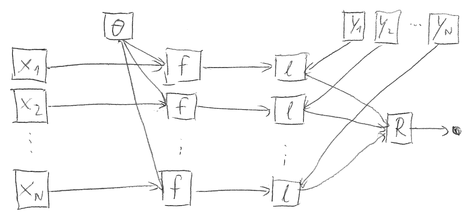
Figure 1: Common computation graph structure in machine learning without batch normalization.
Batch normalization
BN satisfies the following structures (compare Figure 2):
[X]Model & loss function split[ ]SIMD structure (forward pass)[X]Reduction structure (loss) (assuming square or cross-entropy loss)[X]SIMD + reduction structure (loss) (assuming square or cross-entropy loss)
Note that the forward pass is less-structured than in the traditional setting:
\begin{equation*} L(F(\mX, \vtheta), \mY) = R\begin{pmatrix} \ell\left( F_1(\mX, \vtheta), \vy_1 \right) & \dots & \ell \left( F_N(\mX, \vtheta), \vy_N \right) \end{pmatrix}\,. \end{equation*}This is a source of confusion when we attempt to generalize concepts starting from the most structured case (Figure 1).
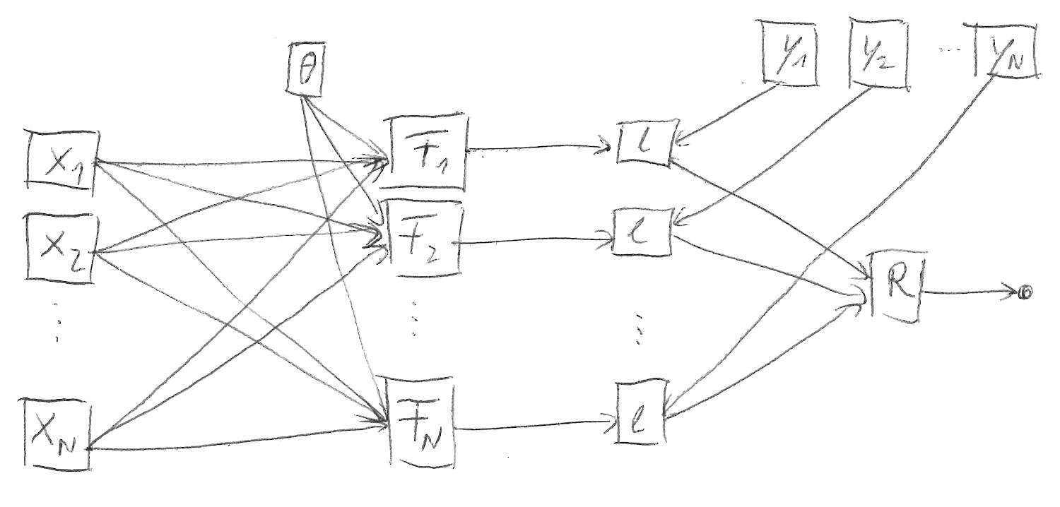
Figure 2: Computation graph structure with batch normalization.
Individual gradients
Individual gradients refer to the gradients with respect to \(\vtheta\) caused by a single sample \((\vx_{n}, \vy_{n})\),
\begin{equation*} \left\{ \nabla_{\vtheta} L(F(\mX, \vtheta), \mY) \Big|_{\substack{\vx_{i\neq n}=\mathrm{const.}\\ \vy_{i\neq n}=\mathrm{const.}}} \right\}_{n=1}^{N}\,. \end{equation*}If all boxes above were checked, they would be proportional to
\begin{equation*} \left\{ \nabla_{\vtheta} \ell(f(\vx_{n}, \vtheta), \vy_{n}) = \left(\mathbf{\mathrm{J}}_{\vtheta} f(\vx_{n}, \vtheta)\right)^{\top} \frac{ \partial\ell(f(\vx_{n}, \vtheta), \vy_{n}) }{ \partial f(\vx_{n}, \vtheta) } \right\}_{n=1}^{N} \end{equation*}up to the reduction factor introduced by \(R\), which will be ignored here for simplicity.
Every member of that set depends only on a single datum \((\vx_{n}, \vy_{n})\). This is why they are called individual (or per-sample) gradients.
They can be computed with automatic differentiation via vector-Jacobian products, but when we apply these in the presence of BN, we obtain
\begin{equation*} \left\{ \left(\mathbf{\mathrm{J}}_{\vtheta} F_{n}(\mX, \vtheta)\right)^{\top} \frac{ \partial\ell(F_{n}(\mX, \vtheta), \vy_{n}) }{ \partial F_{n}(\mX, \vtheta) } \propto \nabla_{\vtheta} L(F(\mX, \vtheta), \mY) \Big|_{\substack{F_{i\neq n}(\mX, \vtheta)=\mathrm{const.}\\ \vy_{i\neq n}=\mathrm{const.}}} \right\}_{n=1}^{N}\,. \end{equation*}These are not gradients caused by individual samples (dependence on \(\mX\) rather than \(\vx_{n}\)), but individual components of the forward pass. It would thus be more adequate to call them per-component gradients.
The component-wise gradient mean is still the overall gradient,
\begin{equation*} \sum_{n=1}^N \left(\mathbf{\mathrm{J}}_{\vtheta} F_{n}(\mX, \vtheta)\right)^{\top} \frac{ \partial\ell(F_{n}(\mX, \vtheta), \vy_{n}) }{ \partial F_{n}(\mX, \vtheta) } \propto \nabla_{\vtheta} L(F(\mX, \vtheta), \mY)\,, \end{equation*}but interpretation of higher moments, like the variance, is unclear.
Conclusion: In the presence of BN, it is possible to apply the same automatic differentiation operations (vector-Jacobian products) required to obtain individual gradients in the traditional setting. But this results in per-component gradients, rather than per-sample gradients. Interpretation of those per-component gradients' statistical higher moments is unclear.
Generalized Gauss-Newton
We have seen in the previous section about individual gradients that the concept of per-sample quantities is replaced by per-component derivatives in the presence of BN. However, we may still be able to exploit structural tricks for quantities that are not defined with respect to individual samples.
One example from BackPACK is the generalized Gauss-Newton's (GGN) diagonal.
Let's start with GGN. It requires a model & loss function split which is present in BN losses,
\begin{align*} \mG(\vtheta) &= \underbrace{ \left( \mathrm{J}_{\vtheta}F(\mX, \vtheta) \right)^\top }_{D \times N C} \underbrace{ \left[ \nabla^2_{F(\mX, \vtheta)} L(F(\mX, \vtheta), \mY) \right] }_{NC \times NC} \underbrace{ \left( \mathrm{J}_{\vtheta}F(\mX, \vtheta) \right) }_{NC \times D}\,, \end{align*}With a (SIMD + reduction) loss, this decomposes into a sum over components,
\begin{align*} &\propto \sum_{n=1}^N \underbrace{ \left( \mathrm{J}_{\vtheta}F_n(\mX, \vtheta) \right)^\top }_{D \times C} \underbrace{ \left[ \nabla^2_{F_n(\mX, \vtheta)} \ell(F_n(\mX, \vtheta), \vy_n) \right] }_{C \times C} \underbrace{ \left( \mathrm{J}_{\vtheta}F_n(\mX, \vtheta) \right) }_{C \times D}\,, \end{align*}(neglecting the reduction factor). Note that, still, we obtain a sum over the batch size. However, each summand depends on all inputs \(\mX\).
Interestingly, this does not affect the computational trick used in BackPACK: If we apply a symmetric decomposition to the loss Hessian,
\begin{align*} \nabla^2_{F_n(\mX, \vtheta)} \ell(F_n(\mX, \vtheta), \vy_n) = \sum_{c=1}^{C} \vs_{nc}(F_n(\mX, \vtheta), \vy_n) \vs_{nc}(F_n(\mX, \vtheta), \vy_n)^{\top} \end{align*}with \(\vs_{nc}(F_n(\mX, \vtheta), \vy_n) \in \sR^{C}\), we obtain
\begin{align*} \mG(\vtheta) &\propto \sum_{n=1}^N \sum_{c=1}^C \left[ \left( \mathrm{J}_{\vtheta}F_n(\mX, \vtheta) \right)^\top \vs_{nc}(F_n(\mX, \vtheta), \vy_n) \right] \left[ \left( \mathrm{J}_{\vtheta}F_n(\mX, \vtheta) \right)^\top \vs_{nc}(F_n(\mX, \vtheta), \vy_n) \right]\,. \end{align*}Still, we can compute \(\mathrm{diag}(\mG(\vtheta))\) of the above expression by backpropagating the vectors \(\{\vs_{nc}\}\) by vector-Jacobian products.
Conclusion:
- It will be possible to support BN in BackPACK's
DiagGGNExactextension, as BN does not interfere with the computational trick (square root factorization of the loss Hessian). As for individual gradients, the per-sample GGNs change to per-component GGNs in the presence of BN, and are thus difficult to interpret (their sum remains interpretable). - Due to the (SIMD + reduction) loss, the GGN is a sum of \(N\) rank-at-most \(C\) matrices. This means that the GGN's rank is at most \(NC\). I've written a paper (dangel2021vivit) that highlights applications of this low-rank structure. Some of the techniques we employ there (for instance computing the GGN spectrum) will still work efficiently with BN, although we excluded it in the paper to preserve the existence of per-sample quantities.
Bibliography
- [ioffe2015batch] Ioffe & Szegedy, Batch Normalization: Accelerating Deep Network Training by Reducing Internal Covariate Shift, 448-456, in in: Proceedings of the 32nd International Conference on Machine Learning, edited by Bach & Blei, PMLR (2015)
- [dangel2021vivit] Felix Dangel, Lukas Tatzel & Philipp Hennig, ViViT: Curvature access through the generalized Gauss-Newton's low-rank structure, , (2021).